Introduction
In this tutorial, we will write a python function that pulls data from Nasdaq Data Link through the tables API, adds relevant columns that are not present in the raw data, updates columns to allow for ease of use, and leaves the data in a format where it can then be used in time series analysis.
Nasdaq Data Link is a provider of numerous different types of financial data from many different asset classes. It provides API’s that allow access from Python, R, Excel, and other methods. It is available to institutional investors as well as individual retail investors.
Nasdaq Data Link Initial Data Retrieval
We will use the data for AAPL for this example. This will give us a data set that requires some thought as to how the splits need to be handled as well as the dividends.
We’ll start with pulling the initial data set, with the first 10 rows shown as follows from the pandas dataframe:

And the last 10 rows:

From left to right, we have the following columns:
- Row number: 0 indexed, gives us the total number of rows/dates of data
- Ticker: The ticker symbol for our data
- Date: In the format YYYY-MM-DD
- Open: Daily open
- High: Daily high
- Low: Daily low
- Close: Daily close
- Volume: Volume of shares traded
- Dividend: Dividend paid on that date
- Split: Split executed on that date
- Adjusted Open: Daily open price adusted for all splits and dividends
- Adjusted High: Daily high price adusted for all splits and dividends
- Adjusted Low: Daily low price adusted for all splits and dividends
- Adjusted Close: Daily close price adusted for all splits and dividends
- Adjusted Volume: Daily volume price adusted for all splits
Data questions
The above information is a good starting point, but what if we are looking for the following answers?
- The data shows a split value for every day, but we know the stock didn’t split every day. What does this represent?
- What is the total cumulative split ratio?
- What is the split ratio at different points in time?
- What is the adjusted share price without including the dividends? This would be needed for any time series analysis.
- What is the dividend dollar value based on an adjusted share price?
- What would the share price be if the stock hadn’t split?
We’ll add columns and modify as necessary to answer the above questions and more.
Assumptions
The remainder of this tutorial assumes the following:
- You have the Nasdaq Data Link library installed
- You have the pandas library installed
- You have the OpenPyXL library installed
Python function to modify the data
The following function will perform the desired modifications:
| |
Let’s break this down line by line.
Imports
First, we need to import the required libraries:
| |
NDL API Key
To gain access to anything beyond the free tier, you will need to provide your access key:
| |
Download data as a dataframe
Moving on to the function definition, we have the command to pull data from NDL. There are two separate APIs - the time series and the tables. The syntax is different, and some data sets are only available as one or the other. We will use the tables API for this tutorial.
| |
In the example above, the fund is an input parameter to the function.
The 'QUOTEMEDIA/PRICES' is the data source that we are accessing.
There are many other arguments that we could pass in the above, including specifying columns, period start date, period end date, and others. Nasdaq as a few examples to get you started:
https://docs.data.nasdaq.com/docs/python-tables
Running:
df.head(10)
Gives us:

Sort columns by date
Next, we will sort the columns by date ascending. By default, the dataframe is created with the data sorted by descending date, and we want to change that:
| |
The inplace = True argument specifies that the sort function should take effect on the existing dataframe.
Now, running:
df.head(10)
Gives us:

Setting the date as the index
Next, we will rename the date column from ‘date’ to ‘Date’, and set the index to be the Date column:
| |
Now, running:
df.head(10)
Gives us:

Calculating splits
The next sections deal with the split column. So far we have only seen a split value of 1.0 in the data, but we’ve only looked at the first 10 and last 10 rows. Are there any other values? Let’s check by running:
| |
And checking the first 10 rows:
df_not_1_split.head(10)
Gives us:

So we now know that the stock did in fact split several times. Next, we will replace all of the 1.0 split values - because they are really meaningless - and then create a new dataframe to deal with the splits.
| |
This gives us:

We will now create a dataframe with only the split values:
| |
Which gives us:
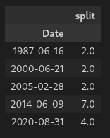
Creating a column for the cumulative split will provide an accurate perspective on the stock price. We can do that with the following:
| |
Which gives us:
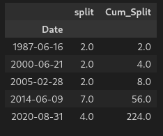
We will then drop the original split column before combining the split data frame with the original data frame, as follows:
| |
Which gives us:
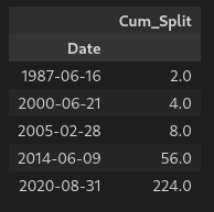
Combining dataframes
Now we will merge the df_split dataframe with the original df dataframe so that the cumulative split column is part of the original dataframe. We will call this data frame df_comp:
| |
We are using the merge function of pandas, which includes arguments for the names of both dataframes to be merged, the column to match between the dataframes, and the parameter for the type of merge to be performed. The outer argument specifies that all rows from both dataframes will be included, and any missing values will be filled in with NaN if there is no matching data. This ensures that all data from both dataframes is retained.
Running:
df_comp.head(10)
Gives us:

Forward filling cumulative split values
From here, we want to fill in the rest of the split and Cum_Split values. This is done using the forward fill function, which for all cells that have a value of NaN will fill in the previous valid value until another value is encountered. Here’s the code:
| |
Running:
df_comp.head(10)
Gives us:
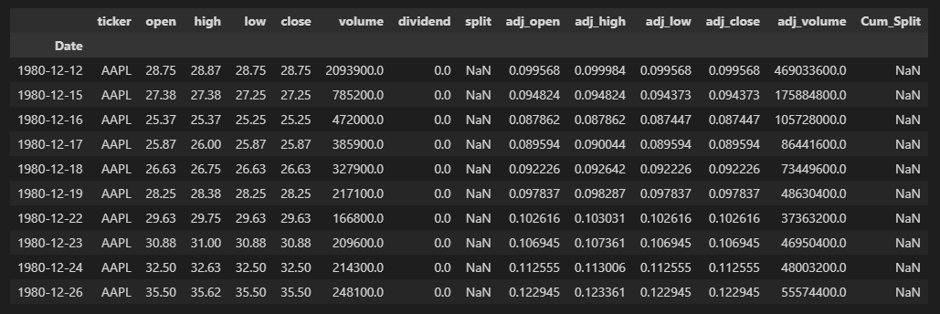
At first glance, it doesn’t look like anything changed. That’s because there wasn’t any ffill action taken on the initial values until pandas encountered a valid value to then forward fill. However, checking the last 10 rows:
df_comp.tail(10)
Gives us:

Which is the result that we were expecting. But, what about the first rows from 12/12/1980 to 6/15/1987? We can fill those split and Cum_Split values with the following code:
| |
Now, checking the first 10 rows:
df_comp.head(10)
Gives us:

With this data, we now know for every day in the data set the following pieces of information:
- If the stock split on that day
- What the total split ratio is up to and including that day
Calculating adjusted and non-adjusted prices
From here, we can complete our dataset by calculating the adjusted and non-adjusted prices using the cumulative split ratios from above:
| |
Included above is the adjusted dividends values. For any time series analysis, not only are the adjusted prices needed, but so are the adusted dividends. Remember, we already have the adjusted total return prices - those come directly from NDL.
Export data
Next, we want to export the data to an excel file, for easy viewing and reference later:
| |
And verify the output is as expected:

Output confirmation
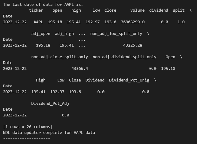
Finally, we want to print a confirmation that the process succeeded along withe last date we have for data:
| |
And confirming the output:
References
https://docs.data.nasdaq.com/docshttps://docs.data.nasdaq.com/docs/tables-1https://docs.data.nasdaq.com/docs/time-serieshttps://docs.data.nasdaq.com/docs/python
